Maxwell’s field equations
By Tyler Housel, Contributing Editor | TLT Lubrication Fundamentals October 2025
Electricity and magnetism are explained using these four classic equations.
The origin of the word electricity comes from the Greek word “elektron” which means “amber.” In antiquity, the Greeks found that rubbing fur against a piece of amber would make it attract feathers and other light objects.1 Meanwhile, “magnet” comes from the lodestones found in the Magnesia region in Thessaly2 that acted on each other with unseen forces and helped navigators find their direction. These strange phenomena invited speculation from scientists, philosophers and charlatans alike. But in 1865, James Clerk Maxwell outshone even Promethius when he solved the twin mysteries of electricity and magnetism by presenting the famous Maxwell equations in “A dynamical theory of the electromagnetic field.”3 The Maxwell equations established the framework for classical electromagnetics and apply to virtually all aspects of the electrified world we live in.
Last month’s TLT Lubrication Fundamentals article noted that electric forces decrease as the square of distance between charged objects (Coulomb’s law) in a close analogy to Newton’s laws of gravity, where the charge (q) plays the same role as mass (M).4
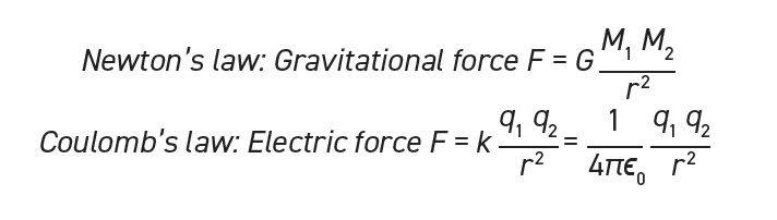
Newton discovered gravity to fit observational evidence of falling bodies on Earth and the motions of heavy bodies such as the moon, sun and planets. However, gravity is weak, and it was impossible to detect the force between two objects on Earth. In Newton’s time, laboratory experiments were limited to measurements of the attraction between one object and the planet itself.
Electric and magnetic forces are much stronger than gravity so experimenters could directly measure the force between two magnets or charged objects in a laboratory. By the mid-1700s scientists including Benjamin Franklin, Joseph Priestly and Henry Cavendish were experimenting with electricity and already began to realize that electricity and gravity appeared to follow similar inverse square laws. As scientists continued to work with charges and magnets, many more secrets of electromagnetism emerged.
Electric field (E)
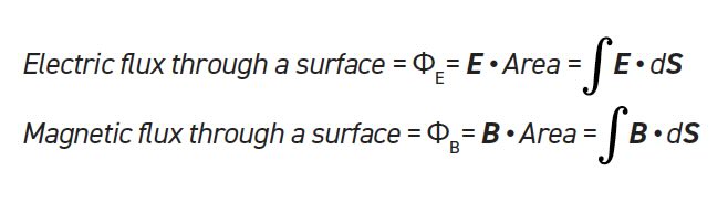
Just like with gravity (last month), Coulomb’s law solves for the electric force on an arbitrary, stationary charged object, and the electric field is the set of all solutions to Coulomb’s law everywhere in space. The electric field (E) measures force (vector) per unit charge (F/q) so the SI units are Newtons per Coulomb (N/C), which also works out to volts per meter (V/m). When we sketch a field as in Figures 1 and 2, the force is generally greater in areas where the lines are closer together and the arrows on the field lines give the direction. Arrows and lines are great for visualizing the geometry of the field, but flux is a more accurate way to work with field equations.
Electric flux (ΦE)
The word “flux” comes from the same root as “flow.” Flow normally relates to physical quantities like air or water. But a static field does not move through time, and it can be strange to think of a field as flowing. Still, the flux measures how much field (E) “flows” through a given area. The orientation is important, and electric flux only measures the component of the field perpendicular to the area. Since the field orientation can change across the surface, we often break the area into smaller areas (dS) and use the dot product to ensure that we are measuring only the perpendicular component at each location (sin 90°=1). Then we add up (integrate) all the flux components across the entire area of interest. The units of electric flux are [(N m2)/C] or [V m] (volt meters, not to be confused with voltmeters).
Magnetic field and flux (B and ΦB)
The previous explanations also apply to the magnetic field (B) and magnetic flux (ΦB). The magnetic field is measured in Amperes per meter (A/m) or Teslas (T) and magnetic flux is measured in Volt seconds (V s) or Webers (Wb). Magnetic field and flux will be discussed later in the article.
Line and surface, open and closed integrals
Mathematicians use a shorthand language to describe complicated phenomena, but casual readers may not notice subtle clues that make a lot of difference. Table 1 is a quick refresher into the forms for line and surface integrals. And remember that the dot product (•) takes only the component of the function perpendicular to the surface element (see Equations and Symbols).
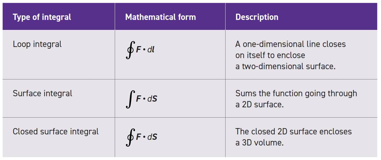
Table 1.
Equations and symbols
This article follows the nomenclature shown in Table 2 which comes from “Physics, Part 2” by David Halliday and Robert Resnick.5 This description of the Maxwell equations, as shown in Table 3, is based on the assumption that there are no dielectric or magnetic materials nearby, and we can ignore relativistic and quantum effects. Maxwell’s equations can be expressed in many other equivalent forms that may look unfamiliar at first.
Table 2
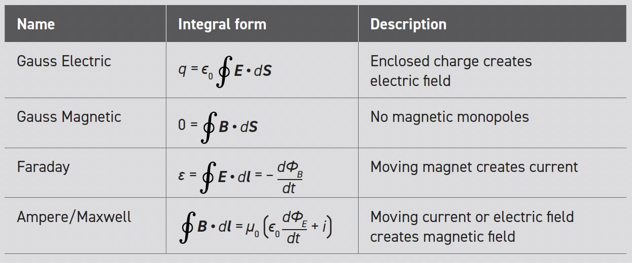
Table 3
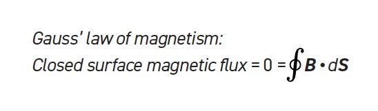
Gauss’ laws for electricity and magnetism
The first and second of what became the Maxwell equations were originally credited to Carl Friedrich Gauss. His law of electricity can be derived from Coulomb’s law and describes the spatial relationship between electric charge and the electric field for any closed volume in space. If the volume contains no net charge, then there is no net electric flux because the electric field lines entering the surface must balance the lines leaving. Two examples are the yellow ovals on the left side of Figure 1 (a two-dimensional representation of three-dimensional space). Although individual charges may be enclosed within the oval, the net internal charge is zero and the incoming and outgoing field lines offset.
On the right side of Figure 1, the red and blue ovals contain charge and, therefore, the net flux is inward (blue) or outward (red). The enclosed charge is proportional to the vector sum of the electric field lines and the permittivity constant (ϵ0) defines the proportionality between the field and charge. Note that the surface can be any shape, so the law is written as an integral across any closed surface (the integral sign with a circle indicates a closed surface).
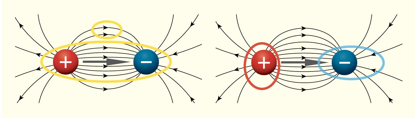
Figure 1. Electric field lines between two charged objects.
Magnetism
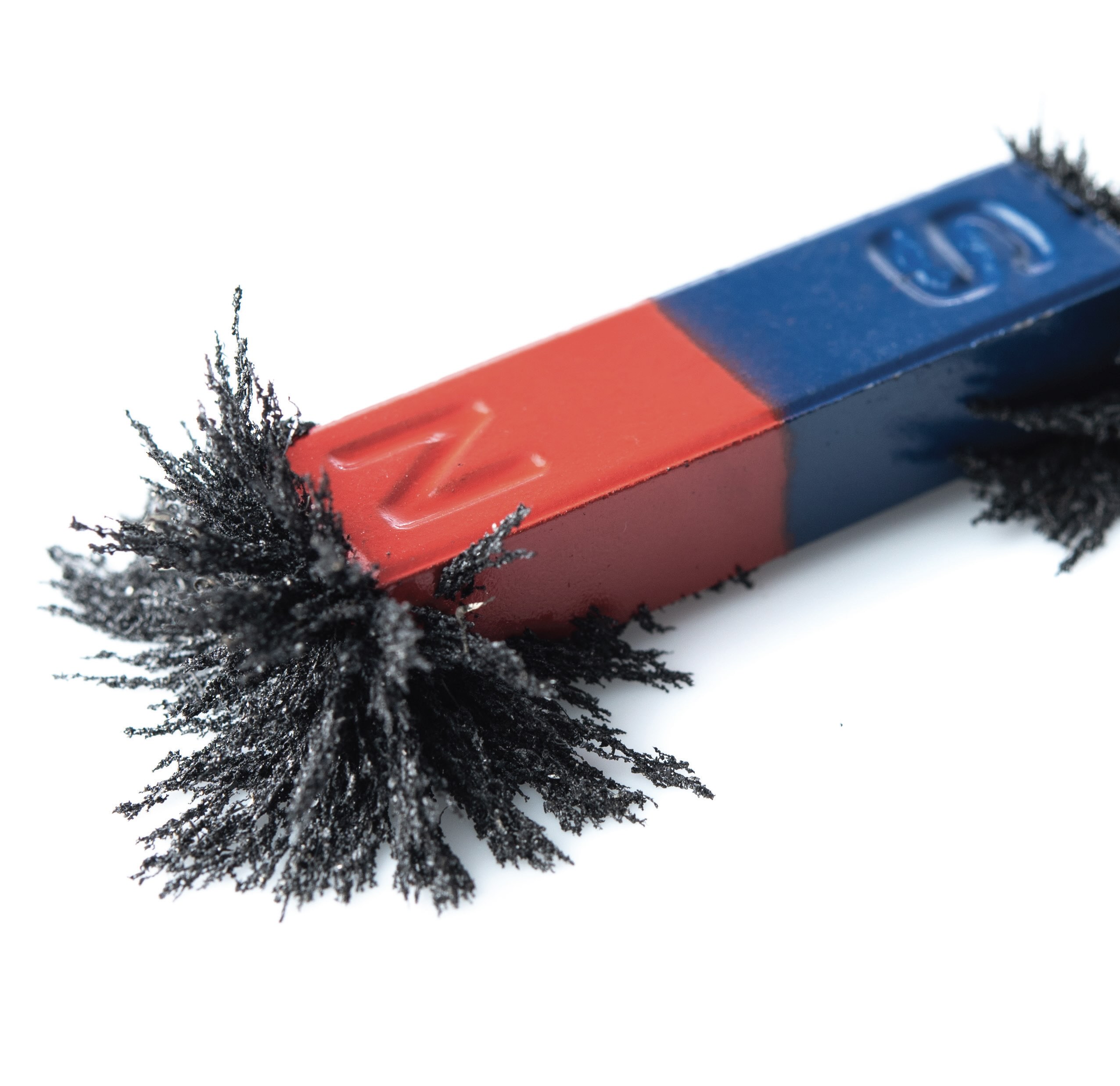
The ends of the magnet are called “North” and “South” to indicate the direction they point to align with the Earth’s magnetic field. Just like electric charges, opposite magnetic poles are attracted to each other and similar poles repel. This means that the North pole of a magnet is attracted to the South pole of Earth’s magnetic field, which is located near the geographic North pole. In the unlikely event that you are using a compass for navigation, the arrow points toward the geographic North; if it spins rapidly, you are probably in a sci-fi movie.
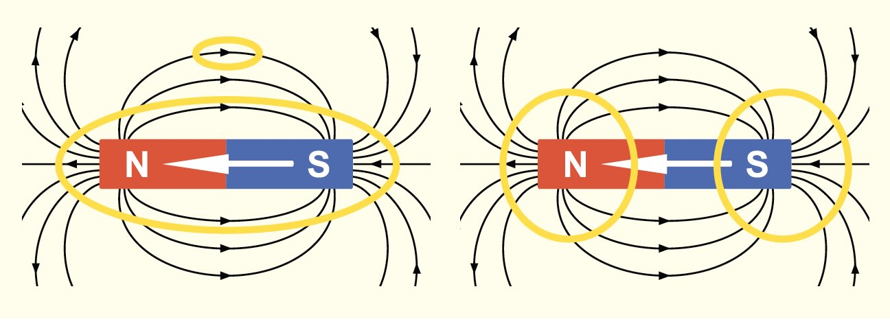
Figure 2. Magnetic field lines of a bar magnet.
At a distance, the electric field of a dipole (see Figure 1) and the magnetic field of a bar magnet (see Figure 2) look identical. Field lines leave from the left side and enter at the right. But one critical difference between electric and magnetic fields is that electric charge can be isolated, but the poles of a magnet cannot. If you break a bar magnet in half, you create two weaker magnets, each with its own North and South pole. Smaller and smaller pieces still have North and South poles. Gauss correctly assumed that it was impossible to isolate a North pole by itself, and his law of magnetism shows that the total magnetic field lines through any volume of space must contain both poles and therefore add to zero. Schematically, the yellow ovals in Figure 2 are all magnetically “neutral” because there is a “return field” within the bar magnet to compensate for the field on the outside. Comparing Figure 1 and 2, electric field lines all go from left to right (positive to negative), but the magnetic field lines inside the magnet flow back in the opposite direction, going right to left (South to North) as shown by the white arrows.
How do magnets work?
Since two South poles repel each other, we might assume any object attracted to the North pole of a magnet would be repelled by a South pole. But many common metals like iron are attracted to either pole. Unmagnetized iron is “ferromagnetic” and can act as either a North or South pole because it has a multitude of tiny magnetic regions within the crystal structure. In a normal (unmagnetized) piece of iron, these regions are randomly distributed and there is no macroscopic magnetic field as shown in Figure 3a. When the North pole of a bar magnet is near a normal piece of iron, it attracts the South poles inside the iron and flips some of the tiny fields to align with the field from the bar magnet (see Figure 3b). And it works the same way for the South pole (see Figure 3c). Quantum physicists call this magnetic alignment “exchange coupling.”
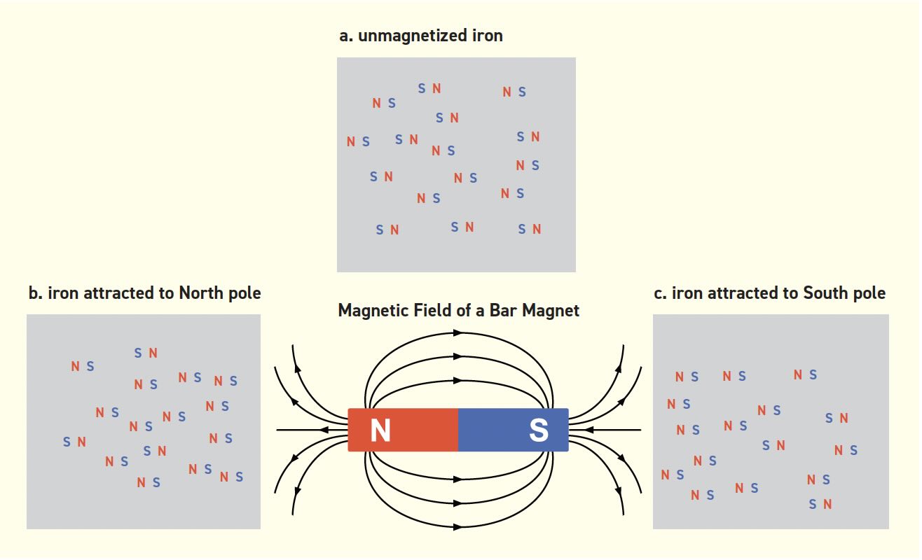
Figure 3. Iron’s random internal magnetic fields align with a magnet’s field.
When the bar magnet is removed, most fields return to their disordered state but often the iron will maintain some memory of the alignment. If the external field is strong enough, iron can become a permanent magnet with the tiny fields aligned in the same direction.6 However, “permanent” may be too strong a word. Magnets can also be demagnetized by other strong fields or by increasing the temperature above the “Curie temperature” where thermal motion randomizes the alignment.
Faraday’s law
Things get much more interesting when charges and magnets are moving. Unlike the first two Maxwell equations, Faraday’s and Ampere’s laws relate electric and magnetic phenomena to each other and have explicit time dependent terms (dt). In the 1830s, Michael Faraday and Joseph Henry contemporaneously discovered that a magnet moving into a loop of wire caused a current in the wire. If the magnet stopped, the current also stopped, and if it was withdrawn, the current reversed. This is called an induction current because the magnet and wire do not touch, and the current was induced by the field around the magnet. Faraday was first to publish his findings, so it’s Faraday’s law forevermore.
Induction requires movement, but it doesn’t matter which one moves. To illustrate, Figure 4 shows two possible positions for a wire loop (gray) near a bar magnet. Observe that there are more magnetic field lines going through the loop at position B, indicating a greater magnetic flux as the loop and magnet get closer together. If the wire moves from A to B, the magnetic flux through the wire loop increases and this induces a current in the wire. If the wire goes back to A, the current reverses.
Faraday’s law shows that the rate of change in magnetic flux through the loop is equal to the electromotive force (ε or EMF) in the wire. If the wire is conductive (closed circuit), electrons will flow around the loop. If the circuit is open, the EMF shows up as a voltage between ends of the wire. It is important to note that this EMF is not “free.” The Ampere/Maxwell law shows that the current in the wire sets up a magnetic field that opposes the motion of the magnet. Hence, we must apply a force to move the magnet into the loop which “pays for” the induced EMF.
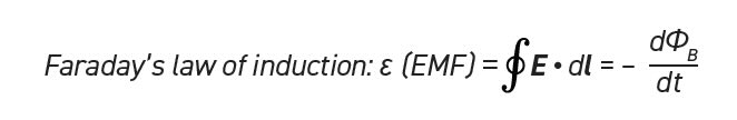
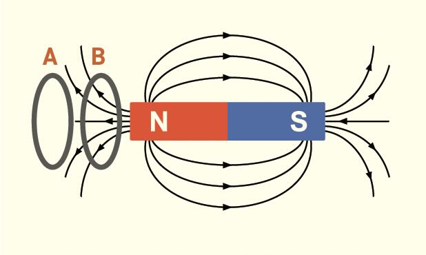
Figure 4. Wire loops (Gray) near a bar magnet.
Ampere’s law
In 1820, Hans Christian Oersted was lecturing on electric currents and noticed that compass needles would deflect a wire when current was flowing. Ampere mapped the forces at different distances with different currents and determined that the emergent magnetic field was directly related to the current flow and perpendicular to the current direction with a proportionality constant known as the (magnetic) permeability constant, μ0 = 1.26x10⁻⁶ H/m. Similar to Gauss’ laws, Ampere’s law only gives a net field value if the current is inside the loop.
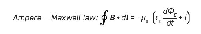
Maxwell started with Ampere’s law but found it necessary to add a second factor to account for time dependent electric fields. If a moving magnet can induce current to flow in a wire, it seems reasonable to think that a changing electric flux would induce changes in the magnetic field. In fact, the second term of the Ampere-Maxwell law has the same form as in Faraday’s law of induction.
Summary
It is impossible to do justice to Maxwell’s equations in 2,500 words or less. The first two equations are pretty straightforward, but when you realize that the last two are mutually entangled, a light literally turns on. Like the funhouse mirrors that continue to reflect each other to infinity, a moving electron causes a magnetic field, which causes an electric field and on and on. These fields continue to interact in a repeating cascade of cause and effect that allow us to see the light from an electron that moved billions of years ago in a galaxy far, far away.
The four classic equations in Table 3 provide (almost) everything you need to know about electromagnetics. Inventors have spent the last two centuries developing increasingly creative ways to harness their power. The next TLT Lubrication Fundamentals article will explain how the electric and magnetic fields cooperate in an electric motor to efficiently transform current into rotational motion.
REFERENCES
1. www.britannica.com/summary/electricity
2. www.etymonline.com
3. Maxwell, J. C. (1865). “A dynamical theory of the electromagnetic field,” Philosophical Transactions of the Royal Society of London, 155, pp. 459-512, https://doi.org/10.1098/rstl.1865.0008.
4. Housel, T. (2025), “Field study,” TLT, 81 (9), pp. 38-41. Available at www.stle.org/files/TLTArchives/2025/09_September/Lubrication_Fundamentals.aspx.
5. Halliday, D. and Resnick, R. (1978), Physics, Part 2, Wiley & Sons, pp. 565-885.
6. www.madehow.com/Volume-2/Magnet.html
Tyler Housel is a technologist for Hnuco Technologies and is based in Lansdale, Pa. You can reach him at tylerhousel@comcast.net.