Complexity in ISFA (in-service fluid analysis): Part XXXIX
Jack Poley | TLT On Condition Monitoring July 2018
Holistic CM in the 21st Century: Part XI
 © Can Stock Photo / enruta
I’ve mentioned technical approaches to data evaluation (essentially the issuing of a report along with a qualified opinion/advisory) numerous times over the years I’ve been writing this column. In this day and age, and as I’ve covered several times in the last few years, expert systems (intelligent agents) are
de rigueur in rendering advisories. There’s way too much information for a human mind to recall and apply consistently time after time. Advisories must be the best they can be: consistently delivered. That’s the essence, the deliverable of fluid analysis, indeed, and all of condition monitoring (CM).
Over a decade ago (2004), I began to revamp my first intelligent agent (expert system) that was designed, crafted and introduced in 1979-1980. In doing so I found numbers of opportunities to
close holes in the logic as well as morph or expand the logic and comments from knowledge I’d since obtained, or that was available from trustworthy, experienced professionals (people I continually consult to enhance the algorithms and advisories provided).
There were numbers of things to do; here are some examples.
1.
Totally new software had to be designed and written.
•
This was a Herculean task. Common business-oriented language (COBOL) had been our platform for nearly 30 years, and we accomplished some very exciting, productive work, including our then-novel intelligent agent, the first ever introduced in the commercial market. It worked very well but was clearly in need of a major update in the 21st Century and—let’s face it—once banks (particularly steeped in COBOL) finally began to be able to abandon it, COBOL programmers, aged or retired, dropped out precipitously. Most labs had no expert system of any kind, though they had tables of boundaries (data limits), at least by the 1990s, for flagging test data. Subsequently the evaluation was done manually by
data analysts. Those who retained COBOL (or DOS) to this day find themselves boxed out of a shot at updating their software in a less than painful, time-consuming process.
•
We chose Java as our platform. It was popular, i.e., there were a plethora of qualified coders, and Java is highly flexible. To date we haven’t regretted that decision. Many who retained older software for data evaluation elected to offload the basic information to a report generator that can avail modern methods, thus, a two-step process.
2.
Coloring became an obsession for data presentation in our reports.
•
One thing that was a must to us was the addition of color in our reports, rating data in a very familiar manner, akin to a typical traffic light, and presenting the data in a field colored accordingly. This provided a quick, logical reference as to the urgency of the posted test values. We eventually added a few more colors to make the rules for data flagging more granular, adding nuance where deemed constructive or the situation demanded. Data coloration represented
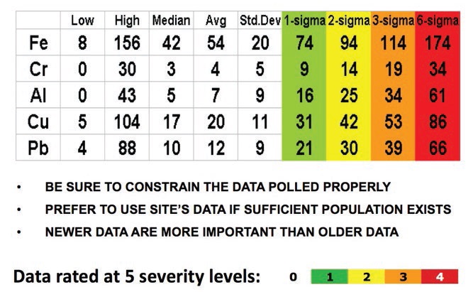
severity of the value. Five severities were initially set up, zero being “normal,” triggering no commentary as to that datum, i.e., excluding it from consideration. Green (notable), yellow (abnormal), orange (high) and red (severe) constituted data rating bins where limits were determined through typical statistical exercises on data conforming to the component type (a minimum requirement). If manufacturer, model and additional, specific component information is available, all the better for relevance and accuracy.
3.
Rating data.
•
Any qualified database, one that has enough data (samples analyzed) to utilize statistical techniques with confidence, will provide the means to set limits.
•
Table 1 shows suggested settings for Severity 1-4 (green through red) using average value + standard deviation (sigma) multiples. This is a common technique, but there is nothing that says one cannot utilize sigma fractions or any other alternative that results in the desired constraints. Over time, limits and trending algorithms are inevitably tweaked to reflect additional data. There also are the notions of normalization for fluid and operating hours, trending beneath limits (run rate) and environmental conditions (exposure to chemicals or dust or water).
Table 1. Data Rating Example Calculating and Setting Limits + Ranges Assign Severity Ratings
4.
Rules that determine advisories.
•
It is important to recognize that, once a statistical range is achieved, and color bins filled, the actual value that determined each color/severity assigned becomes less significant because its overall importance in the data mix has already been defined. Data are then confined to five states, four of which can be represented in rules.
•
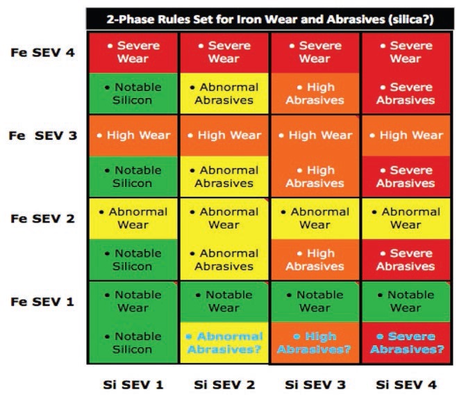
This brings us to pattern recognition, the primary tool of
artificial intelligence. Table 2 is emblematic, a very typical relationship between, say, iron (Fe) and silicon (Si). You might ponder this matrix in the abstract, i.e., irrespective of what type of component the test results (the severities for Fe and Si) originated. There are 16 propositions that are actually “comment slots.” Assuming Fe is often the dominant wear metal in a used lube sample, and that Si is more often than not abrasive in the form of sand-like “dirt,” how would you fill each of these “opportunities” such that all the bases are covered?
•
What do you say when Fe is Severity 4 and Si Severity 1?
•
What do you say when Si is Severity 4 and Fe Severity 1?
•
What comments would you make for the remaining 14 propositions?
•
[Assume nothing else is abnormal so far as available test data.]
•
[Assume this is a routine sample with no special condition reported.]
Table 2. 2-Phase Rule for Fe & Si Wear vs. Abrasives (?)