KEY CONCEPTS
•
Condition monitoring is the process of measuring equipment parameters that can include vibration, temperature and oil condition, among other things.
•
Predictive maintenance uses the data resulting from condition monitoring techniques to predict equipment health and identify when maintenance is needed to prevent expensive equipment failure.
•
Effective predictive maintenance programs reduce needed maintenance, while increasing reliability and reducing costs.
Industry used to rely on two primary equipment maintenance strategies or philosophies: reactive and preventive. Reactive maintenance is simply fixing things when they break down; however, that concept is nearly inconceivable with today’s complex equipment. The next strategy is preventive maintenance, which involved following a scheduled maintenance program.
However, following World War II, industry went beyond the ideas of reactive and preventive maintenance to predictive and proactive maintenance strategies. Predictive maintenance uses sample data to allow for coordinating maintenance programs to predict and respond to equipment failures before they occur. The benefits of this approach include minimizing equipment downtime while also reducing maintenance costs by eliminating unnecessary scheduled maintenance. The key is performing the right tests on the right equipment at the right time to predict when maintenance is needed.
Proactive maintenance involves the use of processes like root cause analysis and failure mode and effect analysis (FMEA) to determine why an asset failed so that the cause might be eliminated, and risk can be managed effectively. Some aspects of predictive technologies also can be used to identify the presence of failure root causes prior to equipment damage taking place. Properly using the technologies and taking appropriate action prior to equipment damage falls into the proactive domain.
Predictive maintenance
Condition monitoring is the process of measuring equipment parameters (e.g., vibration, temperature, lubricant analysis, etc.) to identify any changes that could predict impending equipment failure. Predictive maintenance analysts act on those measurements by using them to predict when maintenance is necessary.
By identifying and detecting equipment failure modes and predicting the rate of failure progression, effective condition monitoring programs allow preventive action to be taken without unplanned downtime. This amounts to predictive maintenance, which uses different technologies, including vibration analysis, lubricant analysis, infrared thermography and ultrasonics, to achieve that goal.
Predictive maintenance strategies can lengthen a machine’s lifespan by addressing issues before they develop into expensive failures, while reducing unnecessary maintenance. Condition monitoring programs are becoming more common as organizations recognize how they can increase reliability and reduce costs.
 If lubricant analysis can identify the failure mode, the next step is identifying the required test.
FMEA. ASTM D7874 standard defines FMEA as, “an analytical approach to determine and address methodically all possible system or component failure modes and their associated causes and effects on system performance.”
1 Effectively applying the FMEA process hinges on an understanding of machine design requirements and equipment operating conditions, which lead to the identification of potential failure modes.
STLE member Lisa Williams, technical solutions specialist at Spectro Scientific in Chelmsford, Mass., notes the first step in applying FMEA is selecting the components to test, then identifying the possible failure modes that are associated with those components. For each component, the causes and effects of each failure mode are identified. Each failure mode is given a severity number (S) and an occurrence frequency number (O) to allow calculation of a criticality number (S x O). The criticality number permits prioritization among the different failure modes and allows determination of whether lubricant analysis can be applied to detect the failure mode.
ASTM D7874 states, “The FMEA methodology prioritizes failure modes based on how serious the consequences of their effects are (S) and how frequently they are expected to occur (O).”
1 ASTM D7874 includes a ranked-number scale for S and O for in-service fluid analysis.
If lubricant analysis can identify the failure mode, the next step is identifying the required test. A detection ability number (D) is used to rank how easily and reliably the failure mode can be detected using the chosen lubricant test.
To cross-check calculations, a comparison of the criticality number and the detection ability number should indicate that the failure modes with the highest criticality numbers also have the highest detection ability numbers. Williams says, “This means the likelihood of catching failure modes with the selected fluid analysis test(s) is high.” In contrast, a mismatch between the two numbers could indicate a weakness in failure mode detection, requiring adjustments to enhance the program.
Determining test methods and sampling frequency. Williams notes that the most intimidating part of developing a condition monitoring program can be selecting the test programs and sampling frequency.
Williams identifies three key points to help in developing this part of a condition monitoring program:
1. Determine which assets are critical. “Critical” can be defined as a certain dollar amount per hour or through safety regulations or other concepts. Whatever are chosen to be critical will be the routinely tested assets.
2. Consider what typically goes wrong on these machines. This will clarify what tests should be run. Williams notes, “80% of machine failures are due to dirty oil,” meaning that a starting point is likely filtration. Moisture (i.e., ppm water) also is a common issue for many applications. A slate of tests can be built over time as process knowledge is developed. Simple screening tests can indicate a need for more advanced tests when the data warrant a deeper investigation.
3. Consider testing frequency. Williams notes, “In general, sample intervals should be short enough to provide at least two samples prior to failure.” Establishing the sampling interval requires data, which can come from a previous failure mode or be generated through a sampling study. Initially, more frequent sampling is the most conservative approach, but sampling frequency can be adjusted over time as more data are gathered.
As not all failure modes can be found through lubricant analysis, it is important to go through the initial steps of identifying all failure modes, applying a criticality number, then deciding if lubricant analysis testing can help with those modes. Williams notes, “The highly analytical process of FMEA can really help identify all failure modes and provide clear direction on appropriate actions that need to be taken.”
Oil analysis testing
Williams says, “When applied correctly, lubricant analysis can be the earliest indicator of impending machine failures.” To develop an effective lubrication program, FMEA can be used to select the correct equipment to test and the right tests to use to evaluate the specific failure modes.
1
TLT Editor Evan Zabawski, senior technical advisor at TestOil, headquartered in Strongsville, Ohio, notes that determining which oil analysis testing method and frequency should be employed for specific equipment depends on the oil analysis program’s goals. Zabawski says that common goals, and the corresponding tests to measure those goals, include:
1. Reducing oil consumption by extending drain intervals. Possible tests for effective timing between intervals include testing for fluid properties with acid number, Fourier transform infrared (FTIR) spectroscopy and viscosity.
2. Extending component life by monitoring wear. Wear tests include elemental spectroscopy and analytical ferrography to test for wear metals.
3. Increasing reliability by predicting impending failures. This can be tested by measuring contaminants by particle count in the oil.
 One of the oil analysis program’s common goals is reducing oil consumption by extending drain intervals. Possible tests for effective timing between intervals include testing for fluid properties with acid number, FTIR spectroscopy and viscosity.
Ed Eckert, technical sales for Burkett Oil Co. in Norcross, Ga., notes that oil analysis laboratories have standard test packages designed for different types of equipment and can assist in determining appropriate sampling intervals. Eckert notes, “Some OEMs have branded programs contracted with oil analysis labs, which have specific test packages and guidelines for sampling of their equipment.” Most oil companies also have programs with their preferred oil analysis lab and can assist in identifying the appropriate testing and sampling intervals.
Testing frequency hinges on a number of variables (e.g., criticality, expense, reliability, efficiency, environment, operating conditions). When testing does not occur frequently enough, problems can be missed, while too frequent testing can make abnormalities difficult to spot or lead to “analysis paralysis” from too much data. Zabawski says, “The most common starting point frequency is either monthly (common in mobile applications) or quarterly (common in stationary applications), with adjustments as deemed necessary,” based on relevant variables.
Zabawski notes that the acquired data must be useful. For example, if oil degradation is being measured, but the oil drain interval is on a short schedule, that test might not provide value. In other words, if the oil drain interval is 500 hours and the expected life of the fluid is 1,500-2,000 hours, then testing the oil degradation is not helpful information for that equipment and process.
Williams notes that successful oil analysis programs have the common theme of having an employee champion who is dedicated to the program and has taken the time to learn about the subject and establish the program within the organization. Without a champion, these programs are difficult to maintain over the long term. Specific training around tribology, failure analysis, oil analysis and ferrography can make the champion successful.
Setting alarm limits
Alarm limits are intended to notify the operator that action needs to be taken. The goal of a limit is to funnel data down and free the operator from laboriously wading through data to find the exceptional situations.
Sometimes OEMs provide information on how to set alarm or condemning limits for fluids; however, Williams and Zabawski note that the OEMs’ recommendations usually do not include all of the parameters needed and might not be useful to a particular application. Zabawski says, “Lubricant supplier limits frequently focus on physical properties and contaminants, but the limits represent the level of contaminants the lubricant can handle and not necessarily the machine, and are affected by operating conditions, predominantly oil drain interval.”
When alarm limits are not set by OEMs, equipment operators can determine alarm limits either statistically based on manufacturer, model or oil type, or they can be trend based. Combining both statistical and trend-based approaches is synergistic. For example, Zabawski notes that a limit tends to be static, only applying as a threshold near the end-of-drain interval, while trend-based limits can spot abnormalities during all the mid-interval samples as well as at the end-of-drain samples. A rule of thumb is to set alarms lower when the oil volume is greater, the drain interval is shorter and/or if the speed or load is lower; however, there is no one limit fits all generalization.
Eckert notes that ASTM D7720 is the most common method for determining alarm limits and “is a good reference to use when developing alarm limits with in-service oil analysis data populations.”
2 Regardless of how the limits are developed, Eckert says, “The best method is the method that accurately represents a ‘normal’ operating condition and does not produce false alarms.”
Williams says, “The calculation of alarm limits should initially be developed based upon a review of a statistically acceptable population of pertinent data along with data associated with failures (if available).” Williams recommends “a sampling study where the machine is under normal operating conditions and gathering at least four or five samples over time to develop a trend.” These data permit the development of averages for normal machine behavior to permit establishing alarms and condemning limits using simple standard deviation techniques. Williams offers the following example: “If the sample data point falls outside of one standard deviation from the average but still within two standard deviations, the sample would be considered marginal—more than two standard deviations away from the average, the sample would be considered critical.”
An initial sampling study is important to understanding a machine’s normal operating conditions. Alarms can then be set through statistics, then refined by applying trending rules to the sample set to permit the recognition of a problem that is worth addressing. Williams notes that the ASTM D7720 and D7669 standards provide more information on how to establish “normal” operating conditions.
2,3
Zabawski says that the usefulness of static alarm limits is limited, as they are based on statistical analysis of a common grouping of machines under similar operating conditions. This means that the limit has merit if the “machine is operated under similar conditions (e.g., load, speed, temperature, ambient environment) for a similar sampling and drain interval.”
4 When any variable changes, that limit loses relevance. Additionally, over-reliance on alarms shifts focus from identifying underlying trends that might truly predict a failure before it occurs, regardless of alarm state.
 The usefulness of static alarm limits is limited, as they are based on statistical analysis of a common grouping of machines under similar operating conditions.
Statistical process control
The usefulness of static alarm limits is limited, as they are based on statistical analysis of a common grouping of machines under similar operating conditions.
Statistical process control
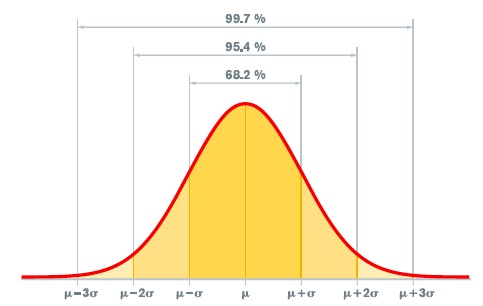
Statistical process control (SPC) is a statistical technique that can be applied to condition monitoring and alarm limits. Zabawski notes that SPC evaluates the distribution of a data set (e.g., the bell curve, where most data points are close to the mean of the whole group). Following ASTM D7720 guidelines, Zabawski says, “The model is based on plus-or-minus three sigma or standard deviations—68.27% of the data set falls into the first sigma, 95.45% within the second and 99.73% within the third.” Following these guidelines, the first warning limit would be set at the value of the second sigma, with the upper control limit set at the value of the third sigma.
While SPC can work well when one sample is taken per drain interval with results about the same value, Zabawski says that when multiple samples are taken throughout the drain interval, the calculation is less useful.
Strategies for trending data analysis
ASTM D7669 provides different strategies for trending data, including cumulative trending, rise-over-run trending, percent change and difference (delta) trending.
3 Table 1 summarizes the four different types of trend analysis and their best uses.
Zabawski states, “Deviations from the normal trend have a far better chance of identifying faults at their earliest stages than any static limit.” According to Zabawski, the most important thing to ensure the success of an oil analysis program is to establish “what is normal” and then observe when it is not “normal.” This means that the program hinges on proper sampling, which is “pulling from a representative, consistent sample point using a proper, consistent procedure at a consistent interval.” This approach will provide the best available data to establish “normal.” Zabawski says, “Consistency is the key, because inconsistencies add noise to the data and make it harder to interpret.”
Eckert notes the saying: “The trend is your friend.” He says the best data for trending hinge on “taking the sample from the same place and the right place on the equipment, as close as possible with time on oil (e.g., every 250 hours oil time), to provide the best data for trending.” Eckert notes that trending data have benefits over just alarm limits as trending “will provide the operator the time to recognize an issue (e.g., wear, contamination, oil condition)
before a flag will be raised with set alarm limits.”
When interpreting sampling data, Eckert says the cumulative trend, which uses a simple plot line on a graph, is likely the most common analysis method (
see Table 1). This method allows the user to visually see a notable increase or decrease in the trend of a single data point or in grouped data. Eckert has found that oil analysis laboratories usually have web-based software available to graphically represent the sample data to permit trending analysis. When there is a high level of confidence in the sampling technique, Eckert finds trend data evaluation more useful in detecting potential problems than set alarm limits. However, when sampling technique confidence is low, trend data might be questionable.
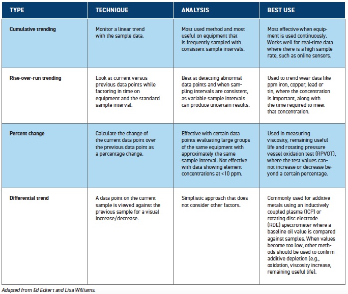 Table 1. Types of data trending analyses
When a good representative data population is established and consistent sampling occurs, Eckert finds trend analysis can be used to determine the optimal drain interval, allowing maintenance to be scheduled at the optimal time. With historical data trends and maintenance records, an operator can use trends to identify when an excessive wear event is happening in a piece of equipment. This information also can be used to determine which equipment part is the source of the wear.
Conclusions
Predictive maintenance programs reduce the need for equipment maintenance, while increasing reliability and reducing costs. However, establishing an effective program requires investment in the process and an understanding of the principles to identify the type of data to collect, as well as the frequency of collection, to arrive at the best possible program for the particular piece of equipment.
REFERENCES
1.
ASTM D7874 (2018), “Standard guide for applying failure mode and effect analysis (FMEA) to in-service lubricant testing,”
ASTM International, West Conshohocken, Pa. DOI: 10.1520/D7874-13R18,
www.astm.org.
2.
ASTM D7720-11 (2017), “Guide for statistically evaluating measurand alarm limits when using oil analysis to monitor equipment and oil for fitness and contamination,”
ASTM International, West Conshohocken, Pa. DOI: 10.1520/D7720-11R17,
www.astm.org.
3.
ASTM D7669 (2020), “Standard guide for practical lubricant condition data trend analysis,”
ASTM International, West Conshohocken, Pa. DOI: 10.1520/D7669-20,
www.astm.org.
4.
Zabawski, E. (Sept. 25, 2017),
Oil Analysis Trending vs. Alarm Limits. Available
here.
ADDITIONAL RESOURCES
1.
Click here.
2.
Click here.
3.
ASTM D6224 (2016), “Standard practice for in-service monitoring of lubricating oil,”
ASTM International, West Conshohocken, Pa. DOI: 10.1520/D6224-16,
www.astm.org.
4.
ASTM D4378 (2020), “Standard practice for in-service monitoring of mineral turbine oils for steam and gas turbines,”
ASTM International, West Conshohocken, Pa. DOI: 10.1520/D4378-20,
www.astm.org.
Andrea R. Aikin is a freelance science writer and editor based in the Denver area. You can contact her at pivoaiki@sprynet.com.