Strategic oil analysis: Time-dependent alarms for extended lubricant lifecycles
Mike Johnson | TLT Best Practices August 2010
Following these strategies allows you to calculate rate of wear generation, a more insightful metric than total wear.

www.canstockphoto.com
KEY CONCEPTS
•
Time-dependent alarms reveal the actual rate of wear per unit of time.
•
The unit of time could be replaced with other incremental units, including production values, miles or operating cycles.
•
As time intervals per oil change increase, the rate of top-up volume should be factored to reflect dilution effects.
Oil analysis is a powerful tool in the machine condition monitoring toolbox—if used properly. Much like other technologies, it performs best within a well-developed plan. When accomplished, a well-devised plan can provide an effective long-term view into the health of any machine with lubricated components.
TLT has provided STLE members with information about test methods, alarm methods and about the best alarm fit for the noted test methods to construct an effective oil analysis approach. The
November 2009 TLT provides an overview that would be a worthwhile preview to this article. This article can be found on the STLE Web site (
www.stle.org).
The 2009 article indicates that there are three common alarm types for grading the underlying problems for sumps and lubricated components. These are statistical (alarms used to identify machine wear problems), absolute (aka aging alarms, used to identify lubricant health and degradation) and percentage-based alarms (used for lubricant health and contamination monitoring).
The focus of Part IV of this five-part series addresses rate of-change (ROC) and volume-compensation alarms. These are common process alarms and could be effectively used to track machine conditions operating under a variety of considerations. When coupled with top-up volume normalization, ROC alarms may help the engineer make decisions about the lubricant’s long-term surface protection characteristics, something difficult to track with routine lubricant-analysis processes. Accordingly, this approach helps with evaluations between high-performance and commodity grade products.
Aside from wear debris analysis, this technique also could be used to measure contamination control effectiveness for hydraulic and circulation systems and improve sump life-cycle management.
TIME-DEPENDENT ALARMS
There are a variety of circumstances under which a ROC or time-dependent alarm is useful. For instance, if the site had a machine that was sputtering through final cycles/hours/units of production and it was necessary to stop the machine before it failed in service, one might use ROC alarms to track the increase in the selected indicator of failure over short blocks of time.
For example, suppose a machine has already produced wear debris indicating an aggressive wear pattern from the routine oil analysis cycle. Perhaps a degraded bearing or gear surface condition is also evident in vibration data. The oil is changed and an inspection conducted to obtain corroborating evidence of a failure symptom. Following conclusion that a repair is pending, the owner wants to squeeze as much time from the machine as possible but wishes to do so safely to avoid collateral damage. An ROC alarm could provide the owner with a wear debris value per unit of time that tells more about the ongoing rate of wear development than an interval reading.
A ROC alarm could be used to measure the rate of oxidative degradation of a large sump volume as well. For instance, as oil ages its rate of degradation often increases. If the oil is hot, wet and/or contaminated with iron or copper wear debris, the rate of decay could accelerate.
Coupled with oil top-up volumes, this method could be used to gauge engine wear for large industrial engines driving ships, trucks and earth-moving vehicles. Particularly, as it pertains to wear debris for engines, the small wear particle size in engine oil analysis is below typical OEM filter element capture size, meaning wear data should be well represented.
WEAR RATES USING ROC ALARM LIMITS
A ROC alarm is applied to a system where the amount of change must be considered relative to the amount of time through which the change occurs.
Consider the data set in Figure 1. This represents the amount of wear that has occurred in a compressor sump during a 24-month period, beginning with an oil change (Month 1) and accounting for routine top-ups that have occurred during the analysis period.
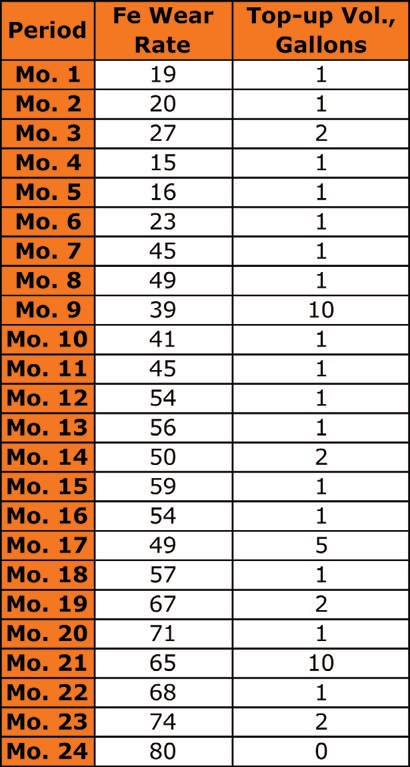 Figure 1. Compressor sump 24-month iron wear and top-up volume record.
Figure 2 shows the iron values plotted out over the period of samples. The plot would seemingly suggest that the wear problem is becoming significant. The black trend line adds credence to the concern. However, the timeline for wear generation should be considered.
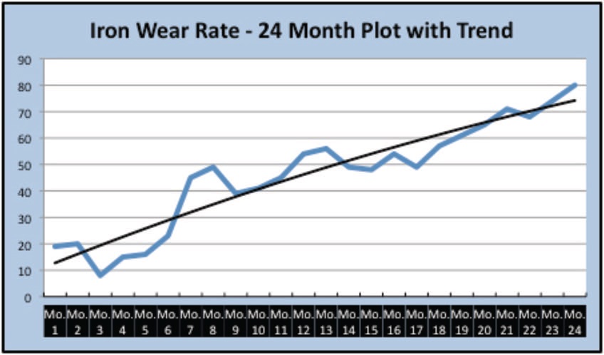 Figure 2. A 24-month wear debris plot and trend.
The chief concern is the ongoing rate of wear generation. Total wear is important but can be misleading. The iron value shown in Month 24 reflects two years of accumulation, less leakage, and does not reflect the extent to which the rate of wear is increasing or not. Figure 3 reflects the same data set adjusted to reflect wear produced per month.
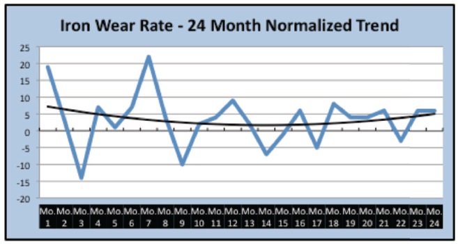 Figure 3. The 24-month wear trend factored to reflect debris generated each month.
After accounting for growth over time, it appears that the rate of wear generation fluctuates between 5 and 30 ppm per month but is steady. The plateau toward the end of the sequence may be explained by a variety of conditions, including weather, operational inconsistencies or operating loads.
The formula for normalization for any type of data set, both process and maintenance measurements, is:
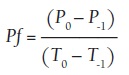
where:
P
f = Factored data point, in this instance iron
P
0 = Current data point
P
-1 = Previous data point
T
0 = Current time period
T
-1 = Previous time period
The values for
P, time period, also could be units of production, tons, miles, years or any other parameter. The actual units must be the same, but the nature of the units can be any parameter defined by the user.
Also keep in mind that the values for V
-1 should reflect an actual condition. In this instance, the iron reading for V
0, which is Month 1, follows an oil change. The wear debris from the previous period is not provided, so the value for V
-1 is zero. If the parameter measured (AN/BN, RPVOT hours, viscosity, etc.) has a definable starting point, use that value. Wear rate for period zero is not measurable.
WEAR RATES & EXTENDED DRAIN INTERVALS
Extension of drain intervals is an expected outcome of improvements in lubrication practices. Mineral oil lifecycles should be extendable by a factor of three to five if the lubricant is maintained in a cool, clean (no atmospheric contaminants and/or wear debris) and dry state. Heat, contaminants and moisture all contribute markedly to oxidation and shortened lifecycles.
Following the example, assume this compressor has a 55-gallon sump and experiences nominal leakage across separator and seals. Rather than change oil at the traditional one-year intervals, the owner is operating on a condition-based change plan. As time passes, total wear in the sump increases, as reflected in the concentration of wear per unit of oil (ppm). When oil is added to the sump, the existing concentration of wear is diluted, being distributed into a larger unit of oil volume. If a significant amount of oil is added, it can appear that the rate of wear is less severe than it truly is. To avoid misinterpretation, the top-up volumes should be factored into the wear rate.
A simple formula to account for added volumes is:
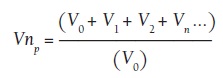
where:
Vn
P = Normalized volume per period
V
0 = Initial volume
V
1 = Period 1
V
2 = Period 2
V
n = Period N
In this example, wear debris is factored by the period (month) to determine the rate of wear. This value can be further factored by the cumulative top-up for that period to provide a monthly wear rate accounting for the total amount of oil added to date.
Treating each monthly data point with the two factors (P
0 * P
f * V
np) enables the reliability engineer to see the ongoing change in light of both time and top-up volume. When applied to the data set from Figure 1, the current plot and trend line, as shown in Figure 4, provides a clearer picture of the machine’s health. Comparing Figures 2, 3 and 4, it is apparent that the wear rate is still tolerable for the machine, but after factoring for top-ups, the rate is twice that perceived from the ROC values. In both instances, the impression of dramatic growth in wear over the 24-month period is lessened.
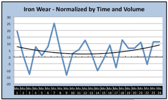 Figure 4. Data set normalized by time and top-up volume.
PRACTICAL APPLICATION FOR NORMALIZED DATA
Figure 4. Data set normalized by time and top-up volume.
PRACTICAL APPLICATION FOR NORMALIZED DATA
Whether a compressor sump, gearbox, engine or other machine type that produces wear debris, factoring data and then applying rate alarms allows the owner to make more informed decisions. Showing the allowable wear rate of <10 ppm per month for the first alarm level overlaid on the graph (
see Figure 5), the reliability engineer can see that the rate of wear is higher than desired and warrants action but is not a cause for dire concern. Options to consider for additional inspections and analysis could include:
•
First, verify that the samples are representative of current conditions.
•
Evaluate with wear debris analysis (ferrography) to identify the wear mode. For cutting wear, improved system cleanliness; for scuffing wear, improved lubricant quality or increased viscosity.
•
Inspect system feed lines to assure lubricant delivery.
•
Verify that the sump temperature is within the suggested operating range.
•
Verify that machine performance is within the expected profile (no misalignment, looseness or load balance issues).
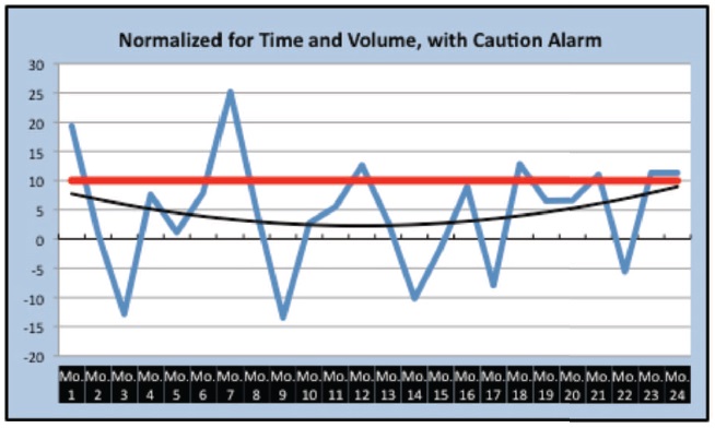 Figure 5. Initial alarm overlaid to contrast actual against allowable wear results.
SUMMARY
Figure 5. Initial alarm overlaid to contrast actual against allowable wear results.
SUMMARY
Machine owners can expect lubricant lifecycles to become extended as they pursue precision lubrication activities. Total wear metals values may give the appearance of a problem where none exists. Total wear debris measurement is most common but does not reflect the state of ongoing machine change and machine health.
To avoid mischaracterizing data, reliability engineers may wish to factor key data points (lubricant health, machine wear debris, contaminant load) to allow for changes over time. Time normalization allows the user to grade the data points for change per unit of time. Sump volume normalization allows the user to grade the data points for change, both for time and for any changes in total sump volume during the whole time increment.
Statistical alarms are particularly helpful if data sets from identical makes and models of a machine type can be grouped to create an expected typical profile for that make and model. Once done, alarm sets can be constructed at 1, 2, 3 and 6 sigma values to provide truly meaningful reporting health interpretation.
Update on machine wear calculation
In this article I provided a simple formula intended to normalize machine wear, accounting for time and top-up (volume), but it proved to be ineffective. There are several models that provide an elegant method to address this question, including these two and many others (
1, 2). Unfortunately, time and resources dedicated to oil analysis within most industrial sites limit the practical applicability of these models. The following is an effort to correct the article error. I welcome your feedback.
Wear over time produces a value for wear rate vs. total wear concentration. Suppose Machine A contains a 100-gallon sump, and sample 1 has produced 100 parts iron during a 450-hour cycle. The wear rate is 100/450=0.222 parts/million/hour (ppm/hr) through 450 hours. If the ensuing sample showed a concentration of 120 parts iron after another 500 hours of run time, then the total iron (120 ppm) divided into the total time (950 hours) produces 0.126 ppm/hr. through 950 hours. This value reflects decreased wear rate even though the total wear concentration is higher. The rate of wear has decreased.
Compensating for changes in sump capacity over time, assume that during the period between the first and second samples, 5 gallons of oil were added and recorded. The 5% increase (in volume) can be used to factor the wear concentration (wear concentration * 1.05 = volume adjusted wear concentration), producing 126 ppm for 950 hours of run time. This reflects a wear rate of (126/950=) 0.132. The rate per hour is slightly higher than the previous example but again reflects a decline in constant wear rate vs. the first example. If the top-up volume was 50 gallons, half the sump capacity, then the factor is 1.5, and the wear rate over time becomes [(120*1.5)/950)=] 0.1894. Again, a rate decline from the first instance.
Please keep in mind:
1.
The change in concentration over time follows an exponential decay. In order for the apparent rate to grow on a straight-line basis, there would have to be increasingly greater wear generated per unit of time to sustain an increase that occurs at a constant rate. This doesn’t normally happen. (
see Reference 1). If the calculated rate/time values don’t level off after a period of time, this is a reflection that the wear rate is accelerating.
2.
Short of a thorough flush of the sump, there is generally residual wear debris remaining following an oil change. A sample with only one hour of time can reflect a rate that may only be reflection of leftover debris. Practically speaking, samples two and following are a better reflection of actual change for time.
3.
If components are wearing normally, the wear rate should decline.
Summarizing:
a.
To determine normalization over time, without any make-up volume, divide the wear concentration by net oil hours for an hourly rate.
b.
To determine normalization with make-up, calculate the volume increase as a percentage and multiply the concentration by the factor, then estimate the rate per Option A (
above).
REFERENCES
1.
Leal, B., Ordieres, J., Capuz-Rizo, S.F. and Cifuentes, P., “Contaminants Analysis in Aircraft Engine Oil and Its Interpretation for Overhaul of the Engine,”
Proceedings of the 9th SWEAS International Conference on Simulation, Modeling and Optimization, pp. 381–386.
2.
Hussin, B. and Wang, W. (2006), “Conditional Residual Time Modeling Using Oil Analysis: A Mixed Condition Information Using Accumulated Metal Concentration and Lubricant Measurements,”
Proceedings of the First International Conference on Maintenance Engineering, pp. 328-336.
 Mike Johnson, CLS, CMRP, MLTII, MLA1, is the principal consultant for Advanced Machine Reliability Resources, in Franklin, Tenn. You can reach him at mike.johnson@precisionlubrication.com
.